

Customer lifetime value is the discounted expected profit a customer will generate over the remaining course of their relationship with a business. For most non-contractual businesses, the strongest starting point for modelling it is a probabilistic buy-till-you-die (BTYD) framework, pairing a latent attrition model like BG/NBD or Pareto/NBD with a Gamma-Gamma monetary model. From there, you set acquisition cost ceilings, segment customers by projected value, and forecast cohort revenue with defensible confidence bounds.
TL;DR:
- Probabilistic BTYD models are best suited for non-contractual, irregular purchase businesses with sufficient transaction volume and feature-poor data.
- Combining BTYD outputs with machine learning models improves accuracy by incorporating rich behavioral and demographic features into CLV predictions.
- Accurate CLV modeling requires at least three transaction fields and a validation process that includes holdout testing and diagnostic checks to avoid overfitting.
- Hierarchical Bayesian shrinkage handles sparse data and cold-start customers effectively by pooling information across segments, while proxy estimates work for completely new customers.
- Proper governance, ethical considerations, and regular model refreshes are essential to making CLV insights actionable and avoiding bias or privacy issues.
Table of Contents
- What is customer lifetime value modelling?
- How do you choose between modelling approaches?
- BTYD in practice: BG/NBD plus Gamma-Gamma
- What data does CLV modelling actually require?
- How do you estimate and debug a CLV model?
- How do you validate CLV estimates and avoid common mistakes?
- How do you turn CLV models into business decisions?
- Advanced techniques for sparse data and richer feature sets
- How Brainiac Consulting builds and governs CLV models
- What ethical and privacy questions does CLV modelling raise?
- How do you handle sparse data and cold-start customers?
- What adopting CLV modelling actually changes for a team
- Building production CLV models with Brainiac Consulting
- Sources
- FAQ
What is customer lifetime value modelling?
Historic CLV simply sums what a customer has already spent, sometimes annualized or averaged across a cohort. It tells you what happened. Predictive CLV estimates what a customer will spend going forward, adjusted for the probability they’re still active, and that distinction is the whole reason modelling exists as a discipline separate from reporting.
Academic treatments of CLV frame it as a disaggregate analogue to discounted cash flow analysis: instead of valuing a company, you’re valuing the future cash flows attributable to one customer relationship, discounted back to present terms, as a foundational review of CLV modelling approaches.pdf) lays out. That framing matters because it tells you what a good CLV model owes you: a defensible present-value number, not just a spreadsheet extrapolation of last year’s average order value.
You need a proper model, rather than a rule-of-thumb heuristic, when any of the following apply:
- Purchase timing is irregular and customers can churn silently, with no cancellation event to flag it (the “non-contractual” problem).
- The business runs on a two-step value realization, where acquisition and monetization happen at different points, and marketing needs to know a lead’s projected worth before it converts.
- Purchase horizons stretch well beyond a single attribution window, so a 30-day lookback tells you almost nothing about true value.
- Finance needs a defensible acquisition cost ceiling by segment, not a company-wide average.
Stakeholders generally expect three concrete outputs from a working model: a per-customer CLV estimate with an uncertainty band, cohort-level revenue forecasts for planning cycles, and a CAC ceiling that varies by acquisition channel or segment. If your current process can’t produce all three, you’re likely still working from historic averages dressed up as predictions.
How do you choose between modelling approaches?
Heuristic methods, average order value multiplied by expected purchase frequency, work fine for early-stage businesses with thin transaction histories or leadership teams that just need a directional number for a board deck. Their weakness shows up fast: heuristics assume every customer behaves like the average customer, which erases exactly the segmentation signal that makes CLV useful in the first place.
Once you have a few thousand repeat customers and a real question to answer (which acquisition channels are worth scaling, which segments deserve retention spend), the choice generally comes down to three model families:
- Probabilistic BTYD models fit non-contractual, discretionary purchase businesses: e-commerce, retail, marketplaces, anywhere customers can simply stop coming back without telling you.
- Survival analysis fits contractual, subscription-style businesses where churn is an observed event (a cancellation, a lapsed renewal) rather than an inferred one.
- Machine learning approaches, gradient-boosted trees or neural networks, fit contexts where you have rich behavioural, demographic, or engagement features beyond transactions alone, and enough volume to train them without overfitting.
The most effective production setups often aren’t pure plays. A common hybrid pattern uses BTYD outputs as engineered features inside a gradient-boosted model, letting the probabilistic layer supply a parsimonious, theoretically grounded baseline while the ML layer absorbs everything else, seasonality, channel, demographic covariates, that a pure latent-attrition model can’t touch. Start with BTYD if you’re transaction-rich but feature-poor. Move toward the hybrid once you have the covariates to justify it.
BTYD in practice: BG/NBD plus Gamma-Gamma
BTYD frameworks split the CLV problem into two independent questions, and treating them separately is the entire reason the approach works. The first question: is this customer still active, and how many transactions will they make in a given future window? The second: given that they transact, how much will they spend? BTYD models answer the first with a latent attrition model and the second with a monetary model, then multiply the two together, as the core BTYD literature describes.
The frequency side uses BG/NBD (Beta-Geometric/Negative Binomial Distribution) or its predecessor, Pareto/NBD. Both assume customers make purchases at a steady individual rate while “alive,” then drop out at some unobserved point, never to return. The model never observes death directly; it infers the probability of it from the gap between a customer’s last purchase and today.
That inference produces three outputs practitioners rely on constantly:
- P(alive): the probability a given customer is still an active buyer, given their purchase history and how long it’s been since their last transaction.
- CET (conditional expected transactions): the expected number of purchases in a future time window, conditional on the customer’s past behaviour and current P(alive).
- DERT or DECT (discounted expected residual transactions): CET summed across all future periods and discounted back to present value, which is the number that actually feeds a CLV calculation.
The monetary side runs on the Gamma-Gamma model, which estimates each customer’s expected average transaction value independently of purchase frequency. That independence assumption isn’t cosmetic. If frequent buyers also happen to spend more per order, the model’s outputs get biased, so a correlation check between frequency and average order value belongs in every diagnostic pass before you trust the Gamma-Gamma layer, as the PyMC-Marketing documentation flags directly.
A worked sketch, in plain numbers: a customer with 8 transactions over about a year, a recent purchase, and typical average order value might have a high P(alive), an expected few transactions over the next year, and a discounted expected residual transaction count somewhat lower than that after discounting. Multiply DERT by the Gamma-Gamma expected monetary value (often close to but not identical to the raw average, since it shrinks noisy individual averages toward the population mean) and you get a present-value CLV estimate for that one customer, with an uncertainty interval around it if you’re running the model in a Bayesian framework.
Before you trust any of these numbers in production, run the standard diagnostic suite: check that the discount rate matches your model’s time unit (annual rates need converting to weekly or daily periods, and CLVTools documents the conversion formulas if you’re working in R), plot predicted versus actual transaction counts by recency-frequency bucket, and confirm P(alive) distributions look sensible rather than clustering suspiciously at 0 or 1.
What data does CLV modelling actually require?
Latent attrition models are famously frugal. At minimum, you need three fields: a customer identifier, a transaction date, and a transaction value. Everything else the model needs, it derives.
From those three columns you compute the RFM-T summary every BTYD implementation expects:
- Frequency: the count of repeat transactions in the observation window (typically excluding the first purchase, which establishes the customer rather than counting as a repeat event).
- Recency (t_x): the time elapsed between the customer’s first and most recent transaction.
- T: the customer’s total age in the dataset, from first transaction to the end of the observation window.
- Monetary: average transaction value, usually the average of repeat transactions only, to keep it consistent with the frequency count.
A two- to three-year transaction history is generally enough for a stable fit, according to practical guidance on CLV modelling implementation, though thinner categories with long purchase cycles (furniture, major appliances) may need more. Returns and refunds deserve a firm rule before you touch the model: either net them against the transaction value or exclude the affected transaction entirely, but pick one convention and apply it consistently, because mixing conventions across a dataset quietly corrupts the monetary model.
Split your data into an estimation period and a holdout period before fitting anything. Fit the model on the estimation window, then check whether its predictions for the holdout window match what actually happened. Skipping this step is the single most common reason production CLV models look great in a notebook and fall apart against real forecasting decisions.
Pro Tip: Run the frequency-monetary correlation check on your RFM-T table before you fit anything. If high-frequency customers are also your highest spenders, segment first and model separately. Applying one Gamma-Gamma model across the whole base will systematically underprice your best customers.
How do you estimate and debug a CLV model?
Maximum likelihood estimation (MLE) is the faster path and works well when you have a reasonably large, homogeneous customer base. Bayesian estimation costs more compute and setup time but pays it back with proper uncertainty intervals on every parameter, and it’s the better choice when segments are small or when leadership needs to see a credible range around a number rather than a single point estimate.
Regularization matters more than most first-time modellers expect. Sparse segments (a new product line, a recently launched region) will produce noisy MLE fits unless you shrink them toward a population-level prior, which is exactly what a hierarchical Bayesian setup does automatically.
On the practical side of fitting:
- Most BTYD implementations use L-BFGS-B or Nelder-Mead optimizers for MLE; if the optimizer isn’t converging, check for customers with only one transaction inflating the boundary cases, and consider trimming or flagging them separately.
- Watch for parameter estimates sitting at the edge of their plausible range (a dropout probability near 0 or 1), which usually signals a data issue rather than a genuine finding.
- Calibration plots, binning customers by predicted CET and comparing to actual repeat purchases in the holdout window, are the fastest way to catch a systematically biased model before it reaches production.
- For Bayesian fits, examine the highest-density intervals (HDIs) on key parameters; an implausibly wide HDI on the dropout parameter usually means you need more data or a more informative prior, not a different model family.
Run every diagnostic at both the individual level and the aggregate cohort level. A model can look reasonable in aggregate while being wildly wrong for specific customers, and that gap is exactly where CAC and segmentation decisions go sideways.
How do you validate CLV estimates and avoid common mistakes?
Validate on the holdout split you set aside during data preparation, not on the same data you used to fit the model. Aggregate checks (does total predicted revenue for the holdout period roughly match actual revenue?) catch gross errors quickly. Individual-level checks (does the model’s ranking of high-value versus low-value customers hold up against what those customers actually spent?) catch the subtler failures that matter more for segmentation.
Overfitting shows up as suspiciously tight confidence intervals on customers with only two or three transactions. The CLVTools validation methodology recommends comparing estimation-period fit against holdout-period fit explicitly, since a model that only looks good on the data it was trained on is a model that will mislead every budgeting decision downstream. Shrinkage and hierarchical priors are the standard remedy.
A quick sanity check worth running on every fit: expected customer lifetime is roughly the reciprocal of the churn rate, so a segment churning at 20% annually implies a roughly five-year expected lifetime. If your model’s implied lifetime is wildly out of step with this back-of-envelope figure, either your churn assumptions or your model specification needs a second look before the number reaches finance.
- Treat every CLV output as a range, not a point estimate, when it feeds a spend decision.
- Prefer the conservative bound of your uncertainty interval when setting CAC ceilings for new channels.
How do you turn CLV models into business decisions?
A revenue CLV number becomes actionable finance can defend once you multiply it by gross margin, converting it into profit CLV. That’s the figure that should actually set your CAC ceiling, not the raw revenue number, which overstates what you can afford to spend on acquisition.
From there, three applications cover most of what marketing and finance teams ask CLV models to do:
- Value-based bidding: feed predicted CLV into ad platforms as a bid signal, so acquisition spend chases customers likely to be valuable rather than customers merely likely to convert once. Platforms that support predictive CLTV commonly combine frequency and monetary components into a single horizon-bounded number for exactly this purpose.
- Audience prioritization: rank existing customers by predicted CLV to direct retention spend, loyalty perks, or account management attention toward the segment that actually moves the P&L.
- Cohort revenue forecasting: aggregate individual DERT and monetary estimates by acquisition cohort to project revenue several quarters out, giving finance a bottom-up number to check against top-down targets.
None of this works if the scores sit in a data science notebook. Push per-customer CLV and P(alive) into your CRM as fields your sales and retention teams can actually filter on, and it starts informing day-to-day prioritization rather than living in a quarterly slide deck. That integration work, more than the modelling itself, is usually where CLV programs stall.
Advanced techniques for sparse data and richer feature sets
Time-invariant covariates (acquisition channel, initial product category) can be baked into a latent attrition model at the individual level, adjusting each customer’s estimated purchase rate and dropout probability from the start. Time-varying covariates, a recent price change, a loyalty program enrolment, are harder to incorporate cleanly and usually push you toward a more flexible model or a hybrid ML layer instead.
Hierarchical Bayesian shrinkage is the standard fix when a meaningful slice of your customer base has only one or two transactions. Rather than fitting each customer (or even each small segment) independently, a hierarchical model pools information across customers, pulling sparse individual estimates toward a population or segment-level mean. The effect is fewer wild, overconfident estimates for your newest cohorts.
- Use time-invariant covariates when the segmenting variable is fixed at acquisition (channel, region, initial basket).
- Reach for hierarchical shrinkage whenever a meaningful share of customers have fewer than three transactions.
- Reach for the BTYD-to-gradient-boosting hybrid once you have enough volume and enough non-transactional features (engagement, support tickets, demographics) to make the extra model complexity worth it.
Pro Tip: Don’t jump straight to a hybrid ML model because it sounds more sophisticated. Run the pure BTYD model first, measure its holdout error, and only add the ML layer if that error is actually too high for the decision it’s informing.
How Brainiac Consulting builds and governs CLV models
Our engagements follow the same repeatable pattern regardless of industry: a data audit to confirm the transaction fields and history depth are usable, a pilot cohort to fit and validate a first model quickly, full estimation and diagnostic passes once the pilot proves out, then production integration into whatever CRM or analytics stack the client already runs.
Deliverables typically include a per-customer CLV table with uncertainty bands, cohort-level revenue forecasts for planning cycles, and CRM-ready audiences segmented by predicted value, all under a governance layer that documents model assumptions and refresh cadence. Our work on improving lead-to-opportunity conversion shows the kind of pipeline impact that comes from pairing predictive scoring with disciplined operational rollout, and the same discipline applies to CLV-driven prioritization.
What ethical and privacy questions does CLV modelling raise?
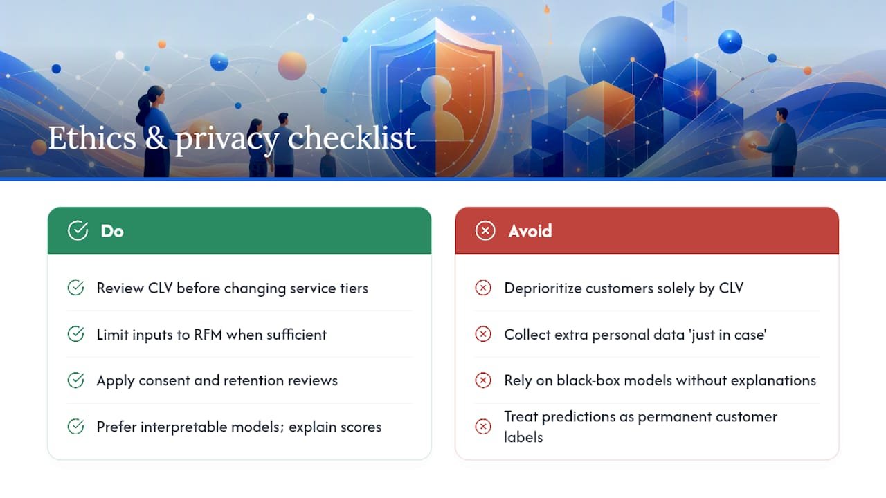
Predicting who’s valuable and who isn’t creates a real risk of treating low-CLV customers worse, slower support responses, fewer offers, degraded service, simply because a model flagged them as unlikely to be worth the investment. That’s a business choice with consequences, not a neutral technical output, and it deserves scrutiny at the point where CLV scores get wired into service tiers rather than just marketing spend.
Data minimization matters here specifically because RFM-T inputs are already sufficient for most BTYD models. You don’t need demographic, location, or browsing data to get a working CLV estimate, so collecting it “just in case” for a model that doesn’t require it is an unforced privacy risk. When you do add covariates, non-transactional signals like engagement or demographic data, that decision should go through the same consent and retention review as any other personal data use, under whatever regional framework applies to your customer base.
Model transparency deserves the same attention as accuracy. A P(alive) score of 0.35 quietly deprioritizing a customer from retention outreach is a decision with real consequences for that person, and teams building on top of CLV outputs should be able to explain, in plain terms, why a given customer landed where they did. That’s harder with a black-box gradient-boosted hybrid than with a BTYD model, whose parameters are individually interpretable, and it’s a legitimate reason to favour the more transparent approach even when the hybrid scores slightly better on holdout error.
Finally, treat CLV predictions as probabilistic guidance for resource allocation, not as a permanent label on a customer. Behaviour changes, and a model trained on last year’s patterns can misjudge a customer who’s simply entering a different life stage or spending pattern. Refresh cadence and human override should be built into the governance process from day one, not added after the first embarrassing misclassification.
How do you handle sparse data and cold-start customers?
A customer with one transaction gives a BTYD model almost nothing to work with, and pretending otherwise produces false confidence rather than a useful estimate. The honest fix is hierarchical shrinkage: pool that customer’s thin history with population or segment-level patterns so their estimate lands near a sensible average rather than swinging wildly based on a single data point.
For genuinely new customers with zero transaction history, no amount of shrinkage helps, because there’s nothing to shrink. The practical workaround is a proxy model: predict expected CLV from acquisition channel, first-order size, referral source, or campaign, whatever signals are available at the moment of acquisition, and treat that as a placeholder estimate until real transaction data accumulates.
Segment-level fallbacks work well as an interim measure too. Assign a new customer the median CLV of their acquisition cohort until they’ve made two or three transactions of their own, then let the individual-level model take over. This avoids the common mistake of either ignoring cold-start customers entirely or assigning them an aggressive value estimate based on a handful of comparable customers who happened to spend heavily.
Whatever approach you choose, flag cold-start estimates explicitly in whatever system consumes them. A CAC ceiling or bidding decision built on a proxy estimate carries meaningfully more uncertainty than one built on eighteen months of transaction history, and treating the two identically in a downstream dashboard is how sparse-data problems turn into budget mistakes.
What adopting CLV modelling actually changes for a team
The biggest shift isn’t technical, it’s what your KPIs reward. Once leadership can see profit CLV by cohort, the conversation moves from “how many leads did we generate” to “what did those leads turn out to be worth,” and that reframing tends to expose channels that looked cheap on a CPA basis but delivered customers who churned within weeks.
Reliable use demands governance most teams underestimate going in: someone needs to own model refresh cadence, someone needs to sign off on which covariates are ethically fair game, and someone needs to be able to explain a low CLV score to a customer-facing team without hand-waving.
Before committing budget to a CLV modelling program, ask honestly: do we have at least a year of clean transaction data, is there a real decision (a bidding rule, a retention budget, a CAC ceiling) waiting on the output, and do we have someone who’ll own the model past the pilot? If any answer is no, fix that first.
— Don
Building production CLV models with Brainiac Consulting
Brainiac Consulting designs and operates the analytics layer that turns a CLV model from a one-off analysis into a system your marketing and finance teams actually run on. Our Atlas AI Operations Platform is built for exactly this: managed AI agents and analytics pipelines that keep per-customer CLV scores, P(alive) values, and cohort forecasts current without a data science team rebuilding the model by hand every quarter.
A typical starter engagement runs as a data audit paired with a pilot cohort: we confirm your transaction data supports a reliable RFM-T summary, fit and validate a first BTYD model against a holdout split, and show you what production integration into Salesforce, HubSpot, or your existing CRM would actually look like before you commit to a full build. From there, our custom AI agents can operationalize the output directly into bidding rules, retention audiences, and finance forecasts, with governance built in rather than bolted on afterward. If you’re weighing whether to build this in-house or hand it to a managed team, our breakdown of managed AI agents versus custom builds is a useful starting point before you scope the engagement.
Sources
For deeper theory, the foundational review of CLV as a disaggregate discounted cash flow measure is worth your time. For implementation, the CLVTools vignette and PyMC-Marketing’s CLV guide walk through fitting and diagnostics in code. For acting on retention once your model is running, see proven customer retention strategies.
FAQ
What Is a Good Customer LTV?
There’s no universal number. A “good” CLV is one that comfortably exceeds your customer acquisition cost, and most businesses target a CLV to CAC ratio well above 1:1 to leave margin for overhead and reinvestment.
What Is a Good CLV to CAC Ratio?
A ratio of 3:1 (CLV three times CAC) is a widely used benchmark for a healthy customer acquisition economy, though capital-intensive or long-payback businesses sometimes accept lower ratios deliberately.
How Do You Calculate Customer Lifetime Value?
In a BTYD framework, you multiply the discounted expected number of future transactions (DERT) by the expected monetary value per transaction from a Gamma-Gamma model, then apply gross margin to convert revenue CLV into profit CLV.
Can You Give an Example of Customer Lifetime Value?
A customer with 8 transactions over about a year, a recent purchase, and typical average order value might have a high P(alive), an expected few transactions over the next year, and a discounted expected residual transaction count somewhat lower than that after discounting, producing a present-value CLV estimate in the low hundreds of dollars once multiplied by expected spend per order.
How Do You Figure Out Customer Lifetime Value for a New Business With Little Data?
Use a segment-level or channel-level proxy estimate until individual transaction histories accumulate, then apply hierarchical Bayesian shrinkage to stabilize estimates as real data starts coming in. Platforms like Brainiac Consulting’s AI analytics services can help set this up as a governed pipeline rather than a one-time spreadsheet exercise.