

Marketing mix modeling is a statistical method that measures how much of your sales or revenue comes from each marketing and non-marketing driver, using aggregate time-series data rather than individual-level tracking. The core outcome it delivers is a decomposition of results into base and incremental volume, so you know exactly which channels earned their spend and where the next dollar should go. Analysts build this with regression techniques, adstock transforms, and response curves to capture how effects build up and fade over time.
TL;DR:
- Marginal ROAS provides more accurate guidance than average ROAS, especially when channels reach saturation and diminishing returns set in.
- Response curves with concave or S-shapes illustrate where each channel hits its saturation point, guiding effective budget reallocation.
- Validating models through live budget shifts and holdout testing is crucial for building trust and ensuring recommendations reflect real-world results.
- Data quality, including weekly granularity over multiple years and segmentation, significantly impacts the reliability of MMM insights.
- Combining regression-based MMM with machine learning techniques via Bayesian methods offers both interpretability and the ability to model complex interactions.
Table of Contents
- What marketing mix modeling actually measures
- How marketing mix modeling actually works under the hood
- The data your marketing mix model actually needs
- Choosing a model structure that matches your business question
- Where marketing mix modeling breaks down
- Building an MMM: the implementation checklist
- What marketing mix modeling looks like in practice
- Validating results and reporting uncertainty honestly
- A brief history of marketing mix modeling
- Marketing mix modeling versus machine learning approaches
- MMM success stories across industries
- Don’s perspective: operational realities and adoption advice
- How Brainiac Consulting operationalizes advanced MMM
- Sources
What marketing mix modeling actually measures
Most stakeholders don’t want a model. They want an answer to a specific question: “If I shift $2 million from television to search, what happens to revenue next quarter?” Marketing mix modeling exists to answer exactly that kind of question, and it does so through four connected outputs.
The first is decomposition. Every model splits total sales into base volume (what would happen with zero marketing, driven by brand equity, distribution, seasonality, and pricing) and incremental volume (the lift attributable to specific marketing and promotional activity). This split alone reframes budget conversations. A brand that assumes its social spend is “working” because sales are up might discover that a large portion of that quarter’s revenue was base demand carried by distribution expansion, not creative.
The second output is channel-level incremental return. This is where marginal ROAS (miROAS) matters more than average ROAS. Average ROAS tells you the historical efficiency of a channel across its entire spend range. Marginal ROAS tells you what the next dollar in that channel will return, which is the number you actually need to make an allocation decision. A channel can show a strong average ROAS while sitting deep in saturation, meaning additional spend there returns far less than the historical average suggests.
Third, response curves visualize this saturation directly. Plotting spend against incremental sales for each channel typically produces a concave or S-shaped curve rather than a straight line, showing diminishing returns as spend increases. Reading these curves correctly is the difference between a model that sits in a slide deck and one that changes a media plan.
Fourth, a working model produces forecasts and scenario outputs, not just historical explanation. Given a defined budget, modern marketing mix modelling can simulate reallocation scenarios and project the resulting sales or revenue outcome before a single dollar moves.
In practice, the outputs stakeholders should expect from any credible MMM engagement include:
- A base-versus-incremental decomposition by time period and by channel.
- Incremental ROI and marginal ROAS estimates for each media and non-media driver.
- Response curves showing where each channel sits relative to its saturation point.
- Carryover estimates showing how long each channel’s effect persists after spend stops.
- Optimization-ready scenarios that translate directly into a revised budget allocation.
Without all five, you have a report. With them, you have a planning tool.
How marketing mix modeling actually works under the hood
Marketing mix modeling differs from media mix modeling and multi-touch attribution in a way that matters for how you interpret its outputs. Media mix modeling is often used interchangeably, though some practitioners reserve the term for models scoped only to media channels, excluding pricing, distribution, and macroeconomic controls. Multi-touch attribution, by contrast, tracks individual user journeys across touchpoints and assigns credit at the person level. MMM works at the aggregate, time-series level, which makes it privacy-resilient but less granular on any single customer’s path. The two methods answer different questions, and treating them as competitors rather than complements is one of the more common strategic errors we see in analytics teams.
Four structural components determine whether an MMM produces trustworthy recommendations or a model that looks fine and misleads.
- Adstock and carryover. Advertising rarely produces its full effect the moment it airs. Adstock transforms model the decay of an ad’s impact over subsequent weeks, and that decay rate varies meaningfully by channel and format. A 15-second social video might decay to half its initial effect within one to two weeks, while a national television campaign or a long-format brand film can carry meaningful effect for six weeks or more. Assuming a single decay rate across channels is a fast way to misattribute credit.
- Response-curve transforms. Once adstocked, spend gets passed through a saturation function, usually a concave (diminishing returns) or S-shaped (threshold-then-diminishing) curve. The shape you choose changes the marginal ROAS estimate at every spend level, so this isn’t a cosmetic modelling choice.
- Additive versus multiplicative structure. An additive model assumes each driver contributes a fixed volume regardless of the others; a multiplicative model assumes drivers interact proportionally, which tends to fit categories where price and promotion amplify or dampen media effects. The order in which you apply adstock and saturation transforms, before or after logging the outcome variable, changes coefficient interpretation, so this decision has to be made deliberately, not defaulted.
- Estimation approach. Frequentist regression (ordinary least squares or ridge/lasso variants) gives point estimates and confidence intervals built on repeated-sampling assumptions. Bayesian estimation instead treats coefficients as distributions, using priors informed by industry benchmarks or historical data, and produces credible intervals through methods like Markov Chain Monte Carlo (MCMC) sampling. For marketing data, which is often short in history and collinear across channels, Bayesian priors help stabilize estimates that frequentist regression alone would leave wildly uncertain. This is increasingly the standard for rigorous MMM programs that need to quantify how confident they actually are in a given ROI estimate, not just report a single number.
Pro Tip: Don’t assume a standard half-life for adstock decay across your channel mix. Tune decay rates by channel and even by creative length, then validate the settings against a holdout period rather than trusting a textbook default.
The mechanics matter because they compound. A model with the wrong saturation shape and an average adstock rate can still produce a plausible-looking chart while feeding you a marginal ROAS that’s off by a wide margin, and nobody downstream will know until the reallocation fails to deliver.
The data your marketing mix model actually needs
An MMM is only as reliable as the data feeding it, and this is where most first attempts stall. The standard recommendation is weekly cadence data spanning two to five years of history, long enough to capture seasonal cycles and enough variation in spend to estimate response curves with confidence.
Statistical Signal: Placement or campaign-level inputs consistently produce more actionable insights than channel-only aggregates, but they also introduce noise and multicollinearity that require deliberate handling during data preparation.
Five categories of variables belong in almost every model:
- Outcome data: weekly sales, revenue, or another primary business KPI, ideally at the same granularity as your spend data.
- Marketing inputs: spend and impressions by channel, including offline media that’s easy to overlook (out-of-home, radio, sponsorships).
- Price and promotion: average selling price, discount depth, and promotional calendars, since these frequently explain more variance than marketers expect.
- Distribution: store count, e-commerce availability, or points of distribution for physical goods categories.
- Macro controls: seasonality indices, holidays, weather where relevant, category growth rates, and competitor activity where available.
On data provenance: first-party data (your own CRM, point-of-sale, and media platform exports) is the most reliable because you control its definition and consistency over time. Second-party data, shared by partners like retailers or agencies, needs careful reconciliation since definitions of “impression” or “spend” can differ across sources. Third-party data, industry benchmarks, syndicated panel data, or macroeconomic series, fills gaps but should never anchor your core estimates without validation against your own numbers.
Granularity creates a genuine trade-off. Channel-level data (total TV, total search) gives you stability and fewer parameters to estimate, but flattens meaningful variation, like the difference between prospecting and retargeting search campaigns. Campaign or creative-level data gives sharper insight but multiplies your parameter count and risks overfitting on a limited number of weekly observations. The practical fix, used across mature MMM programs, is stacking segments, combining geography and product line, for instance, to multiply effective data points while preserving the behaviour within each segment, then modelling the stacked panel with a structure that can borrow statistical strength across groups.
Choosing a model structure that matches your business question
Not every marketing question needs the same model architecture, and building the most complex version available is a common way to waste budget on a model nobody trusts. The right starting point is the decision the model needs to support.
A simple channel-level model, media spend by category regressed against sales, works well for annual planning conversations and high-level budget reallocation across major channels.
Nested or structural models earn their complexity when you need to link short-term sales effects with longer-term brand health. A nested design might feed a brand-tracking index (awareness, consideration, purchase intent) as an intermediate outcome that then flows into a sales model, capturing the reality that a display campaign might not move this week’s revenue but moves the awareness metric that predicts next quarter’s revenue. This structure directly answers the “does upper-funnel spend matter” question that a single-KPI sales model can’t.
Segmentation strategy should follow your business structure, not an arbitrary desire for granularity:
- Geographic segmentation works well for retailers or franchises with regional media buying, and it multiplies observations for hierarchical modelling.
- Product-level segmentation matters when different product lines have genuinely different buyer behaviour and marketing mixes.
- Cohort segmentation (new versus existing customers) helps separate acquisition effectiveness from retention or loyalty effects, which often respond to entirely different channels.
The trade-off running underneath all of this is explainability against granularity against overfitting risk. A model with forty parameters estimated on 104 weeks of data will fit the training period beautifully and generalize poorly. A model with six parameters will generalize reliably but may miss real distinctions your stakeholders care about. The discipline is matching model complexity to the decision at hand and to the actual number of independent observations your data supports, not to how sophisticated the model can theoretically become.
Where marketing mix modeling breaks down
MMM is a correlational tool dressed in causal language, and that gap is the single most important limitation to understand before you present results to a CFO. The model estimates statistical relationships between spend and outcomes; it doesn’t observe causation directly. If an important driver, a competitor’s price cut, a supply shortage, a shift in consumer sentiment, is omitted from the model, its effect gets absorbed into whichever included variable correlates with it, quietly distorting your channel estimates.
Several practical pitfalls compound this risk:
- Overfitting, building a model with more parameters than your weekly data can reliably support, produces flattering historical fit and unreliable forecasts.
- Multicollinearity, when two channels move together (television and paid search often launch simultaneously in a campaign), makes it statistically difficult to separate their individual contributions.
- Poor transform choice, wrong adstock decay or the wrong saturation curve shape, systematically biases marginal ROAS in one direction.
- Data gaps, missing weeks, inconsistent spend definitions across platforms, or an unrecorded price change, quietly corrupt the base decomposition.
The fix isn’t to abandon MMM. It’s to treat it as one instrument in a measurement portfolio rather than a solitary oracle. A well-run measurement program pairs the aggregate, strategic estimates MMM produces with in-market validation, geo experiments that hold out specific markets from a spend increase, randomized lift tests, calibrated multi-touch attribution for tactical, campaign-level decisions, and brand-lift studies for upper-funnel effects that sales data alone won’t capture.
Pro Tip: Before presenting MMM results to leadership, run one small, controlled budget shift in a real market and compare the actual sales response to what your model predicted. A model that survives contact with reality earns trust that a slide deck never will.
Building an MMM: the implementation checklist
Operationalizing marketing mix modeling is a sequence, not a single build event, and skipping steps to get to a headline number faster is exactly how models lose stakeholder trust six months later.
- Define KPIs and decision rules first. Before touching data, agree on what business outcome the model needs to explain (revenue, units, leads) and what decisions the output will drive: annual budget splits, quarterly reallocation, or campaign-level go/no-go calls. This determines your required granularity before you collect anything.
- Gather and validate every data source. Pull weekly spend, impressions, sales, pricing, promotion, and distribution data across your full historical window. Reconcile definitions across platforms (a “click” in one ad platform’s export isn’t always defined the same way as another’s), standardize units, and build a defensible approach to imputing missing weeks rather than silently dropping them.
- Choose transforms and model structure deliberately. Select adstock decay ranges by channel type, choose response-curve shapes based on category knowledge and prior campaigns, and decide additive versus multiplicative structure based on how price and promotion interact with media in your category.
- Train, validate, and stress-test. Fit the model, then validate with holdout periods the model never saw during training, and backtest against known historical events (a launch, a stockout, a price change) to see whether the model’s story matches what actually happened. Run robustness checks by re-estimating with slightly different time windows to confirm your key coefficients don’t swing wildly.
- Run scenario optimization. With a validated model, simulate specific reallocation scenarios, shifting budget between channels, testing different total spend levels, and translate the output into a concrete recommendation: move $X from channel A to channel B, expect incremental revenue of $Y within a stated confidence range.
- Operationalize the cadence. A model refreshed once a year and then filed away delivers a fraction of its potential value. Build dashboards that surface updated response curves and marginal ROAS on a recurring schedule, and establish the cross-functional handoff, media planning, finance, and analytics reviewing the same numbers together, so recommendations actually reach the people who control budget.
A few operational details make each of those steps go faster:
- Keep a versioned log of every model iteration and the data snapshot it used, so results are reproducible when someone asks “why did the number change?”
- Assign a named owner for data pipeline health; MMM breaks quietly when an upstream spend feed changes format and nobody notices for three weeks.
- Build the scenario-planning interface for non-technical stakeholders before the model is “finished,” since early feedback on how planners want to interact with outputs shapes what the model needs to produce.
This is also where the modern shift in MMM tooling matters most. Analysts increasingly need software-enabled workflows that support near-real-time scenario planning rather than a static annual report, which changes how you scope steps 5 and 6 from the start.
What marketing mix modeling looks like in practice
Consider a packaged goods brand running national television alongside a growing digital budget. A response-curve analysis shows the television channel sitting well past its efficient spend range, marginal ROAS has dropped to a fraction of its average, while a paid search line sits comfortably below saturation with room for additional spend to generate strong incremental return. The model doesn’t say “television doesn’t work.” It says the next television dollar is far less productive than the next search dollar, which is a reallocation decision, not a channel-elimination decision.
Trade promotions present a different challenge: sizing incremental lift against cannibalization. A retailer running a temporary price discount sees a sales spike, but part of that spike is pantry-loading, customers buying now who would have bought at full price later, rather than genuinely new demand. A well-specified MMM separates the incremental lift attributable to the promotion from the portion that simply pulled forward future sales, giving trade marketing teams a defensible number instead of a gross sales bump that overstates true impact.
Nested models earn their complexity in categories where brand consideration moves slower than purchase. A financial services brand might feed a tracked consideration metric into a sales model, revealing that a portion of upper-funnel spend that looks unproductive on a same-quarter sales basis is actually building the consideration base that converts over the following two to three quarters.
On magnitude: expect conservative numbers. Meta-analytic research on advertising effectiveness finds that average short-term advertising elasticities run lower than older industry benchmarks assumed, though internet advertising tends to show relatively higher elasticity than traditional formats. Set stakeholder expectations around that reality before the first model output lands in an executive’s inbox.
Validating results and reporting uncertainty honestly
A model’s credibility depends less on its R² than on whether it survives contact with reality. Holdout validation, testing the model against weeks it never saw during training, and backtesting against known historical events form the statistical baseline. In-market validation, small controlled budget shifts or geo lift tests compared against the model’s predicted response, is what actually earns stakeholder trust, because it demonstrates the model’s recommendations hold up outside the spreadsheet.
Governance matters as much as statistics here. Version every model build with its data snapshot, require peer review of transform choices and coefficient interpretation before results go external, and build a formal stakeholder sign-off step so finance and media planning teams have seen and challenged the numbers before they become a budget decision.
When you present results, show the range, not just the point estimate. Bayesian credible intervals communicate this naturally: instead of reporting “search ROAS is 3.2,” report “search ROAS is likely between 2.6 and 3.9, with 3.2 as the most probable value,” and state the scenario assumptions (flat competitive activity, no major price change) that the forecast depends on.
- Refresh cadence should match how fast your media mix and pricing actually change, quarterly at minimum for most categories, faster for high-velocity retail or e-commerce.
- Monitor for structural breaks, a new competitor entrant, a channel algorithm change, a macro shock, that would invalidate historical relationships the model relies on.
Pro Tip: Present one scenario your model got wrong alongside the ones it got right. A team that shows its model’s limits, not just its wins, gets more budget approved on the next recommendation, not less.
A brief history of marketing mix modeling
Marketing mix modeling traces back to econometric sales-response modelling developed in the 1960s, when packaged goods companies first applied regression techniques to separate the sales impact of price, distribution, and advertising. For decades it remained the domain of specialized econometric consultancies running annual, spreadsheet-heavy engagements for large advertisers with the budget and patience for a multi-month build cycle.
The 2000s brought broader adoption as computing power made more complex model structures, adstock transforms, nested KPI designs, feasible outside a handful of boutique firms. Digital media’s rise complicated the picture: as channels multiplied and campaign cycles compressed, the annual-report cadence of traditional MMM started to feel mismatched to how fast media plans actually changed.
The most consequential shift has happened over the past several years, driven by two forces converging at once. Privacy regulation and the decline of third-party tracking pushed marketers toward measurement methods that don’t depend on individual-level cookies, and MMM’s aggregate, time-series approach was already built for that world. At the same time, cloud computing and open-source Bayesian modelling frameworks made faster, more automated model refreshes practical for teams without a dedicated econometrics department. The result is the modern MMM landscape: software-enabled, scenario-ready, and increasingly built to support decisions made in weeks, not the annual cycle that defined the discipline for most of its history.
Marketing mix modeling versus machine learning approaches
Traditional MMM, built on regression with explicit adstock and saturation transforms, has one major advantage that newer machine learning approaches struggle to match: interpretability. When a regression coefficient tells you television contributed a specific incremental volume, you can explain that number to a CFO in one sentence and defend the assumption behind it.
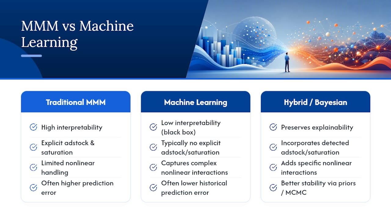
Machine learning approaches, gradient boosting, random forests, or neural network based models applied to the same marketing data, can capture more complex, non-linear interactions between channels and controls that a standard regression structure might miss. They often produce lower prediction error on historical data. But that flexibility comes at a real cost: many of these models function as a black box, making it difficult to isolate a clean, decomposable “this channel contributed this much” statement, which is precisely the output most budget conversations need.
The practical answer for most analytics teams isn’t choosing one over the other; it’s a hybrid. Some practitioners use machine learning methods to identify which interactions and non-linearities matter, then build those specific relationships into an interpretable Bayesian regression structure rather than deploying the black-box model directly for budget decisions. This preserves the explainability that stakeholders need while capturing complexity that a purely additive or multiplicative model would miss. Bayesian estimation itself sits in this middle ground: it’s still fundamentally a regression framework, but the priors and MCMC sampling it uses borrow techniques from broader statistical machine learning to produce more stable estimates from limited marketing data than classical frequentist regression alone would deliver.
MMM success stories across industries
Retail and consumer packaged goods remain the categories with the longest MMM track record, largely because they generate the high-frequency sales and pricing data the method needs. A grocery or beverage brand running MMM alongside promotional calendars can typically separate genuine incremental lift from pantry-loading within a single planning cycle, giving trade marketing teams a number finance actually trusts when negotiating retailer deals.
Financial services and insurance brands have leaned into nested, multi-KPI designs because their sales cycles are long and consideration matters more than same-week conversion. Feeding a tracked brand consideration metric into a sales-outcome model lets these categories justify upper-funnel spend that a single-KPI sales model would flag as unproductive, even though it’s building the pipeline that converts two or three quarters later.
Telecommunications and subscription businesses use MMM to manage the tension between acquisition and retention spend, since the two often compete for the same budget pool but respond to entirely different channels and creative approaches. Cohort segmentation, splitting new versus existing customers, lets these brands see acquisition and retention effectiveness as separate curves instead of one blended, misleading average.
Across all three categories, the common thread in successful programs isn’t the sophistication of the model. It’s the discipline of validating results against real budget shifts before scaling a recommendation across the full media plan, which is the practice that turns a statistical exercise into a decision leadership actually acts on.
Don’s perspective: operational realities and adoption advice
The technical debates around MMM, Bayesian priors, transform choices, model structure, matter less than most analytics teams assume once you get into the room with finance. What actually changes the planning conversation is a credible range instead of a false-precision point estimate. Finance teams don’t distrust MMM because the math is wrong; they distrust it because too many teams present a single ROAS number with unwarranted confidence and no visible seams.
The real blocker is rarely statistical. It’s organizational: media planners who see the model as a threat to their judgment, and a finance team unwilling to act on a recommendation nobody can explain in plain language. The fix is involving both groups before the first model output exists, not after.
Our advice for faster deployment: start with a simple channel-level model, validate it against one real budget shift, and earn trust before building the nested, nine-parameter version everyone eventually wants. Complexity that isn’t earned gets ignored.
— Don
How Brainiac Consulting operationalizes advanced MMM
Building a credible marketing mix model is one project. Keeping it fed with clean data, refreshed on a cadence that matches your media plan, and connected to the dashboards your finance and media teams actually open every week is a different, ongoing challenge, and it’s the one most in-house teams underestimate.

Consultants can handle that operational layer end to end: data engineering pipelines that keep spend, sales, and pricing feeds clean and current; Bayesian MMM builds that produce credible intervals instead of false-precision point estimates; scenario-planning tools that let planners test a budget shift before committing it; and dashboard integrations with platforms like Salesforce, HubSpot, and Tableau so results reach the people who make allocation decisions, not just an analytics team’s shared drive. Clients typically see faster scenario turnaround and budget recommendations that finance can act on more clearly without a follow-up meeting. If you’re ready to move from an annual MMM report to a live, scenario-ready operations platform, request a consultation and we’ll walk through what a working model looks like for your specific media mix.
Sources
For deeper technical grounding, the Think with Google MMM handbook and its companion modelling guidebook cover transform selection and data preparation in detail. Gartner’s MMM overview tracks the shift toward scenario-ready measurement, while Ipsos MMA’s primer explains how MMM complements attribution and experimentation.